Putting Data on a Map
Often, we want to put data in a pandas dataframe directly on a map - here’s how!
[1]:
import numpy as np
import pandas as pd
import xarray as xr

import ptolemy as pt
[2]:
ds = xr.tutorial.load_dataset("air_temperature")
ds["lon"] = ds.lon - 360  # change from degrees_east to centered at prime meridian
grid = ds.air.isel(time=1)
url = "https://d2ad6b4ur7yvpq.cloudfront.net/naturalearth-3.3.0/ne_110m_admin_0_countries.geojson"
[3]:
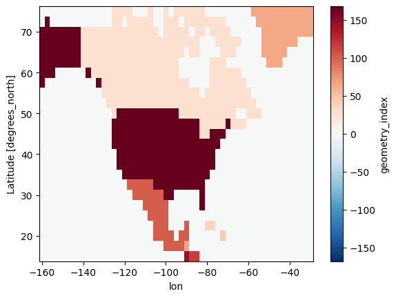
r = pt.Rasterize(like=grid)
r.read_shpf(url, idxkey="adm0_a3")
idxr = r.rasterize(strategy="majority", verbose=True)
idxr.plot()
[3]:
<matplotlib.collections.QuadMesh at 0x2dba961e440>
[4]:
idx_map = {v: int(k) for k, v in idxr.attrs.items() if int(k) in np.unique(idxr)}
idx_map
[4]:
{'CAN': 27,
 'CUB': 37,
 'DOM': 44,
 'GRL': 65,
 'GTM': 66,
 'MEX': 102,
 'NIC': 116,
 'SLV': 144,
 'USA': 168}
[5]:
df = pd.DataFrame(
    {
        "adm0_a3": ["USA"] * 2 + ["MEX"] * 2,
        "year": [2015, 2020] * 2,
        "data": [15, 20, 5, 10],
    }
)
df
[5]:
| adm0_a3 | year | data | |
|---|---|---|---|
| 0 | USA | 2015 | 15 |
| 1 | USA | 2020 | 20 |
| 2 | MEX | 2015 | 5 |
| 3 | MEX | 2020 | 10 |
[6]:
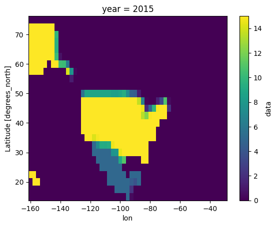
ds = pt.df_to_raster(df, idxr, "adm0_a3", idx_map, coords=["year"])
ds
[6]:
<xarray.Dataset>
Dimensions:  (lat: 25, lon: 53, year: 2)
Coordinates:
  * lat      (lat) float32 75.0 72.5 70.0 67.5 65.0 ... 25.0 22.5 20.0 17.5 15.0
  * lon      (lon) float32 -160.0 -157.5 -155.0 -152.5 ... -35.0 -32.5 -30.0
  * year     (year) int64 2015 2020
Data variables:
data (lat, lon, year) float64 nan nan nan nan nan ... nan nan nan nan[7]:
ds.data.sel(year=2015).plot()
[7]:
<matplotlib.collections.QuadMesh at 0x2dba980f340>

Applying data to multiple raster layers
In many applications, we actually have a single raster layer for each shape we are rasterizing which corresponds to the percent of the grid cell covered by that shape. That was shown in our introduction tutorial, which we repeat here:
[8]:
r = pt.Rasterize(like=grid)
r.read_shpf(url, idxkey="adm0_a3")
idxr_w = r.rasterize(strategy="weighted", verbose=True)
[9]:
idxr_w.sel(adm0_a3="MEX").plot()
[9]:
<matplotlib.collections.QuadMesh at 0x2dbab0fef20>
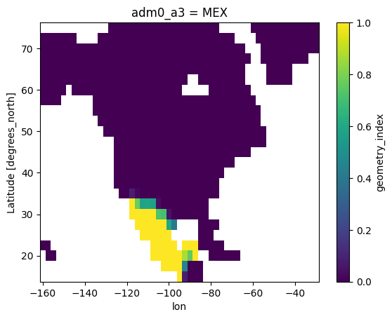
You can then apply data to your map based on these weighted raster layers directly.
[10]:
ds_w = pt.df_to_weighted_raster(df, idxr_w, extra_coords=["year"], sum_dim=["adm0_a3"])
ds_w.data.sel(year=2015).plot()
[10]:
<matplotlib.collections.QuadMesh at 0x2dbab1e5900>
Getting data from a map (Zonal Statistics)
Using the tools developed so far, we can also get data corresponding to different shape areas (i.e., zonal statistics). For that, we need to provide the data to extract and mapping information from the index rasters.
[11]:
pt.raster_to_df(ds, idxr, idx_map=idx_map, idx_dim="adm0_a3", func="max")
[11]:
| year | adm0_a3 | data | |
|---|---|---|---|
| 0 | 2015 | MEX | 5.0 |
| 1 | 2015 | USA | 15.0 |
| 2 | 2020 | MEX | 10.0 |
| 3 | 2020 | USA | 20.0 |
[12]:
pt.raster_to_df(ds, idxr, idx_map=idx_map, idx_dim="adm0_a3", func="sum")
[12]:
| year | adm0_a3 | data | |
|---|---|---|---|
| 0 | 2015 | MEX | 170.0 |
| 1 | 2015 | USA | 2685.0 |
| 2 | 2020 | MEX | 340.0 |
| 3 | 2020 | USA | 3580.0 |
Similarly, raster_to_df() supports weighted rasters but these need to be applied carefully as they can overlap multiple shapes
[13]:
pt.raster_to_df(ds, idxr_w, func="max")
[13]:
| year | adm0_a3 | data | |
|---|---|---|---|
| 0 | 2015 | BLZ | 0.849057 |
| 1 | 2015 | CAN | 8.571428 |
| 2 | 2015 | GTM | 2.745902 |
| 3 | 2015 | MEX | 5.000000 |
| 4 | 2015 | USA | 15.000000 |
| 5 | 2020 | BLZ | 1.698113 |
| 6 | 2020 | CAN | 11.428571 |
| 7 | 2020 | GTM | 5.491803 |
| 8 | 2020 | MEX | 10.000000 |
| 9 | 2020 | USA | 20.000000 |
[14]:
pt.raster_to_df(ds, idxr_w, func="mean")
[14]:
| year | adm0_a3 | data | |
|---|---|---|---|
| 0 | 2015 | BLZ | 0.003986 |
| 1 | 2015 | CAN | 0.628625 |
| 2 | 2015 | GTM | 0.017635 |
| 3 | 2015 | MEX | 0.731777 |
| 4 | 2015 | USA | 12.021734 |
| 5 | 2020 | BLZ | 0.007972 |
| 6 | 2020 | CAN | 0.838166 |
| 7 | 2020 | GTM | 0.035269 |
| 8 | 2020 | MEX | 1.454658 |
| 9 | 2020 | USA | 16.067691 |