Introduction

Here we are giving a brief introduction to rasterizing shapefiles by rasterizing country ids into a given grid.

[1]:

import pyogrio as pio
import xarray as xr

import ptolemy as pt

Data

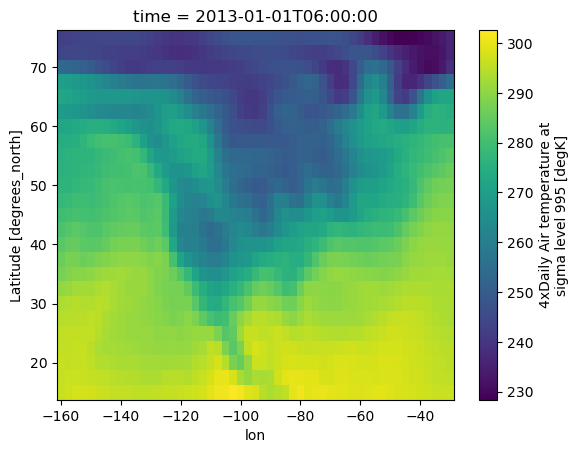
We generally begin with gridded data that we want our future raster to look like. Let’s take an example from xarray looking at some data over North America.

[2]:

ds = xr.tutorial.load_dataset("air_temperature")
ds["lon"] = ds.lon - 360  # change from degrees_east to centered at prime meridian
grid = ds.air.isel(time=1)
grid.plot()

[2]:

<matplotlib.collections.QuadMesh at 0x14c211730>

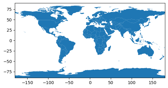
../_images/notebooks_introduction_4_1.png

We can then pull out a shapefile dataset for country borders

[3]:

url = "https://d2ad6b4ur7yvpq.cloudfront.net/naturalearth-3.3.0/ne_110m_admin_0_countries.geojson"

[5]:

# let's take a look
ax = pio.read_dataframe(url).plot()
ax.set_xlim(-180, 180)
ax.set_ylim(-90, 90)

[5]:

(-90.0, 90.0)

../_images/notebooks_introduction_7_1.png

Rasterize with Ptolemy

The basic steps are to great a Rasterize object, tell it what shapefile you want to rasterize, and what strategy you want to use to do the rasterization.

Because ptolemy is built on excellent packages like rasterio which link into GDAL, we get some basic rasterization approaches for ‘free’ - these are basically just pass throughs to the `gdal_rasterize <https://gdal.org/programs/gdal_rasterize.html>`__ functions and include

centroid: each pixel is assigned the shape element which overlaps its center
all_touched: all pixels touched by shape elements are assigned those elements, depends on the order shape elements are assessed

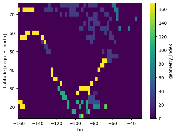
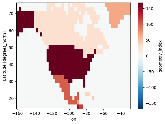
[6]:

r = pt.Rasterize(like=grid)
r.read_shpf(url, idxkey="iso_a3")
idxr_c = r.rasterize(strategy="centroid", verbose=True)
idxr_c.plot()  # idxr_c is an xr.DataArray

[6]:

<matplotlib.collections.QuadMesh at 0x155dbfd40>

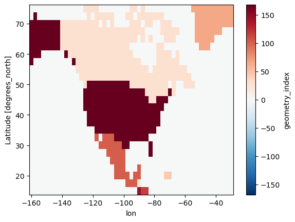
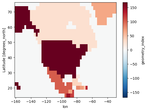
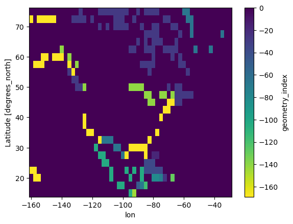
../_images/notebooks_introduction_9_1.png

We can also use an ‘all-touched’ approach

[7]:

r = pt.Rasterize(like=grid)
r.read_shpf(url, idxkey="iso_a3")
idxr_at = r.rasterize(strategy="all_touched", verbose=True)
idxr_at.plot()

[7]:

<matplotlib.collections.QuadMesh at 0x156a0a0f0>

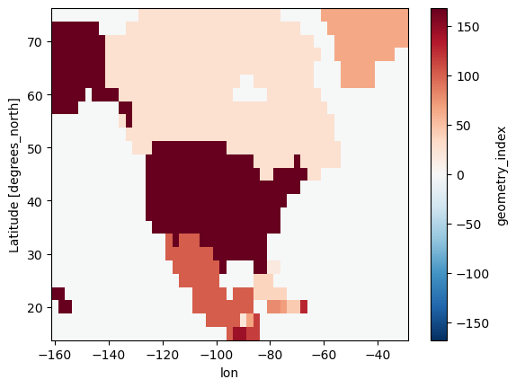
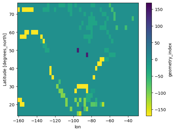
../_images/notebooks_introduction_11_1.png

and see the differences

[8]:

(idxr_c - idxr_at).plot(cmap="viridis_r")

[8]:

<matplotlib.collections.QuadMesh at 0x156a6f1d0>

../_images/notebooks_introduction_13_1.png

Advanced Rasterization Approaches

Hybrid

The hybrid approach tries to get the best of both worlds from centroid and all_touched. It performs both rasterizations, preferring centroids, but then filling in missing cells from the all touched approach.

By implementation, it does the following

mask_hybrid = mask_centroid + np.where(mask_centroid == 0, mask_all_touched, 0)

[9]:

r = pt.Rasterize(like=grid)
r.read_shpf(url, idxkey="iso_a3")
idxr_h = r.rasterize(strategy="hybrid", verbose=True)
idxr_h.plot()

[9]:

<matplotlib.collections.QuadMesh at 0x156bdd1c0>

../_images/notebooks_introduction_15_1.png

[10]:

(idxr_h - idxr_at).plot(cmap="viridis_r")

[10]:

<matplotlib.collections.QuadMesh at 0x156bb71d0>

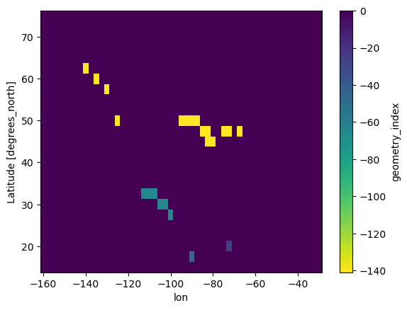
../_images/notebooks_introduction_16_1.png

[11]:

(idxr_h - idxr_c).plot()

[11]:

<matplotlib.collections.QuadMesh at 0x156b6b170>

../_images/notebooks_introduction_17_1.png

Majority

Sometimes one or more shapes overlap into the same grid cell. ptolemy offers methods to calculate which shape has the largest proportion of the cell and assign the cell that shape value. Notice in the below map that the country borders are ‘clean’.

[12]:

r = pt.Rasterize(like=grid)
r.read_shpf(url, idxkey="iso_a3")
idxr_m = r.rasterize(strategy="majority", verbose=True)
idxr_m.plot()

[12]:

<matplotlib.collections.QuadMesh at 0x158c13170>

../_images/notebooks_introduction_19_1.png

[13]:

(idxr_m - idxr_h).plot(cmap="viridis_r")

[13]:

<matplotlib.collections.QuadMesh at 0x158bf7f80>

../_images/notebooks_introduction_20_1.png

It can be the case that empty area takes up the most space of a cell, but we still want to assign that to a shape with data. We have a method for that!

[14]:

r = pt.Rasterize(like=grid)
r.read_shpf(url, idxkey="iso_a3")
idxr_m_ignore = r.rasterize(strategy="majority_ignore_nodata", verbose=True)
idxr_m_ignore.plot()

[14]:

<matplotlib.collections.QuadMesh at 0x158ba8ec0>

../_images/notebooks_introduction_22_1.png

[15]:

(idxr_m_ignore - idxr_m).plot(cmap="viridis_r")

[15]:

<matplotlib.collections.QuadMesh at 0x158ebf350>

../_images/notebooks_introduction_23_1.png

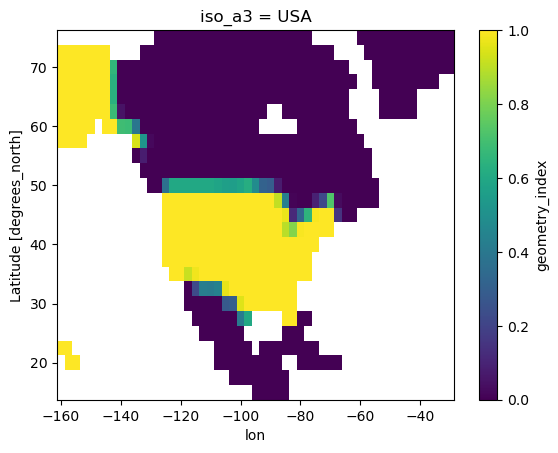
Percent of area rasters

The final approach we have is to simply tell you the fraction of area in each grid cell taken up by a shape as rasterized. This produces a much larger array, since it includes a new dimension with size N_shapes.

[16]:

r = pt.Rasterize(like=grid)
r.read_shpf(url, idxkey="iso_a3")
idxr_w = r.rasterize(strategy="weighted")

[18]:

idxr_w.sel(iso_a3="USA").plot()

[18]:

<matplotlib.collections.QuadMesh at 0x15903fd40>

../_images/notebooks_introduction_26_1.png

[19]:

idxr_w.sel(iso_a3="MEX").plot()

[19]:

<matplotlib.collections.QuadMesh at 0x159018bc0>

../_images/notebooks_introduction_27_1.png